Wire-flexure thermal decoupling, with mixed constraints using flexures and rubber for dynamics stiffness and damping.

Problem description

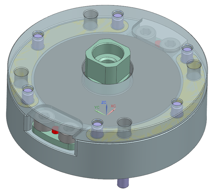
Figure 1 shows a concept for a magnetically levitated positioning stage, which it is to position a wafer with sub-micron accuracy.

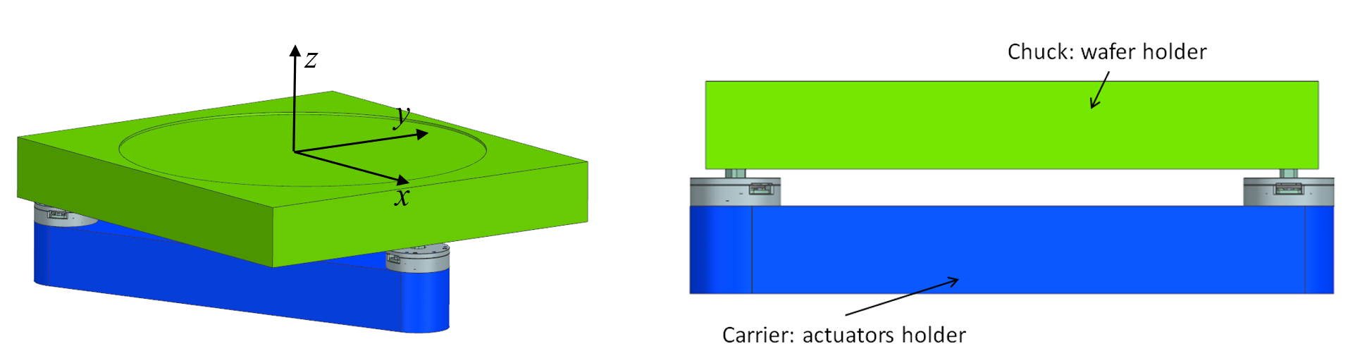
Figure 1: Moving assembly of a magnetically levitated positioning stage.

The main function of the moving assembly, chuck and carrier, is to carry a wafer and to position it in 3 DOF, z, rx and ry, using magnetic actuators, e.g. Lorentz motors or reluctance actuators. In this concept the coils are attached to the moving part, the actuator holder in Figure 1, and the magnets are stationary. This generally leads to a lower moving mass. However, the moving coil concept introduces heat in the moving part the wafer holder. Additionally, vibrations induced in the actuation direction need to be reduced. 

Principle

The moving part is split in two parts, a wafer holder and carrier holder, connected by several flexures and rubber pads. Slender flexures, particularly wire-flexures, provide a thermal resistance because of their small cross sectional area and length. In the concept the flexures are arranged such that they constrain the three in-plane DOFs x, y and rz, while rubber pads constrain the z, rx and ry direction, in the glassy state at high frequencies. This is important for high bandwidth motion control. At low frequencies the rubber is compliant, but the resulting motion between actuator holder and wafer holder is measured and actively compensated for by the magnetic actuators at the wafer holder. The rubber is a thermal resistance and provides damping of induced vibrations, particularly in the actuation directions. 

Design

Three flexure assemblies, one shown in Figure 2, are oriented as shown in Figure 3, to constrain the in-plane x-, y- and rz-directions. In this case a flexure assembly comprises two collinear wire-flexures which constrain the y-direction. For applications with a larger variation of the temperature an exact constrained single wire-flexure per assembly should be considered. Here the two wire flexures are not prone to buckling, whereas a single wire flexure, prone to buckling, might need to be reinforced jeopardizing the thermal resistance. The flexure body, shown in Figure 4, has two lobes to be connected with rubber sheets for damping. Two rubber sheets are mounted in the single flexure assembly as shown in Figure 6. Given the relatively large contact area with the rubber, the z-direction is well constrained in particular for higher frequencies. Combined one flexure assembly imposes two constraints. Therefore the wafer holder has six constraints with respect to the Carrier. Thanks to this, thermal expansion of the Carrier will not introduce stress/deformations on the Chuck. The arrangement of the wire-flexures also creates a thermal center at the center of the wafer, therefore the wafer holder won’t be affected by homogenous thermal expansion of the carrier. Note that the rubber must be properly glued to its interfaces (or vulcanized), in order to prevent micro slip which will introduce hysteresis. The complete flexure assembly is shown in Figure 5.

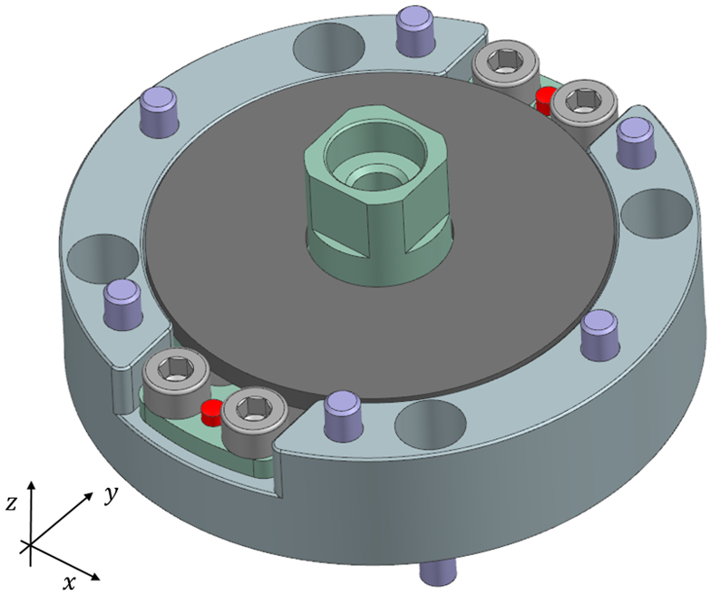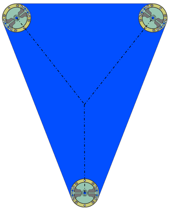Figure 2: Flexure in its holder.	Figure 3: The three flexures that connect Chuck and Carrier.

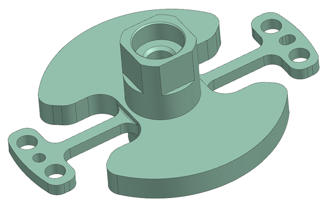Figure 4: The flexure body has two lobes to be connected with rubber sheets for damping.	Figure 5: The complete flexure assembly.

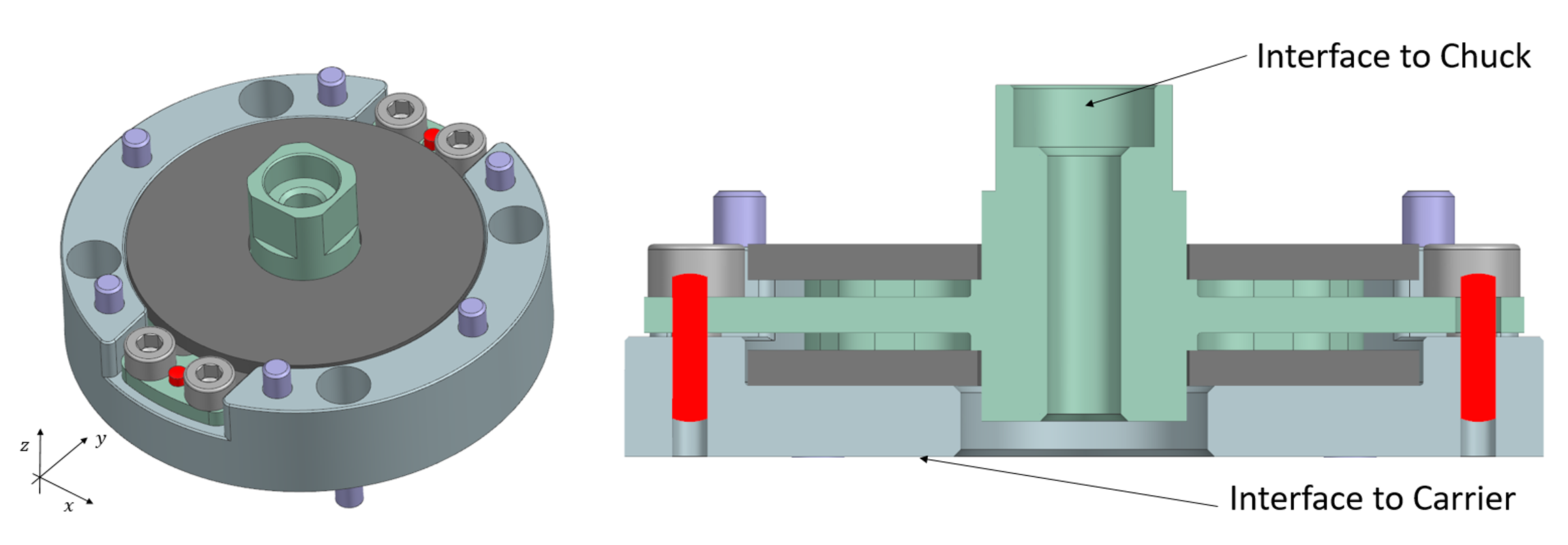
Figure 6: Coordinate system and cross section of the flexure assembly.

Calculations

The following chapters describe the steps that lead to define the initial model for the flexure assembly. These are relatively simple calculations that allow to make the initial design choices. These choices are necessary in order to set up the model that will be used for a more accurate analysis (for instance by using FEA methods) which will allow to optimize the design.

Static analysis

The goal of the static analysis is to make sure that the stiffness of the flexure assembly is according to the requirements: the stiffness in the constrained direction should be higher than a minimum value to keep the first eigenfrequency above the minimum required, while the stiffness in the compliant direction should be small enough to keep the thermally induced deformations low. For this case the maximum stiffness in the compliant direction $x$ should be bound at $6 \:10^6 N/m$ and at the same time a minimum stiffness of $1 \:10^8 N/m$ for the stiffness in $y$-direction is required. The stiffness in $z$-direction may statically be very low, because the $z$-direction will be actively adjusted. 

Figure 7 shows the relevant parameters that will be used for the analysis:

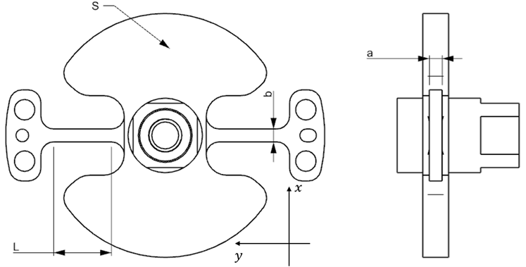
Figure 7: Relevant dimensions for the flexure calculations.

The values are: $L=9mm, a=4mm, b=1.2mm, S=697mm^2$.

The stiffness of the flexure assembly is a parallel combination of the stiffness of the flexure itself with the stiffness of the rubber sheets. However, for the stiffness in the  direction the flexure stiffness is much higher than the stiffness of the rubber sheets, therefore the rubber stiffness in neglected. A good approximation is to consider only the most compliant part of the beam (length $L$ ); following the definitions given in Figure 7, defining $A$ the section of the flexure beam of length $L$ and given that the material chosen is stainless steel AISI 304L (Young’s modulus $E=200 GPa$ ):

$k_y=2\frac{EA}{L}=2.1 \:10^8 N/m$

(1)

As for the stiffness in $x$, both flexure beams will contribute in parallel. For one beam, the model is shown in below Figure 8:

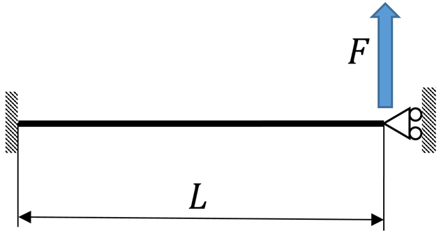
Figure 8: Model of the flexure to evaluate the stiffness $k_x$ .

Considering that there are two beams in parallel, the contribution of the flexure is:

$kf_x=2\frac{12EI_z}{L^3}=3.8 \:10^6 N/m$

(2)

Given that $x$ is the compliant direction of the flexure, the contribution of the rubber in $y$ might be not negligible; the resulting stiffness in $x$ is the parallel of the flexure and the two rubber sheets, which are loaded with a shear stress. For each rubber sheet, the stiffness is:

$kr_x=\frac{G_rS}{h}$

(3)

where $G$ is the shear modulus, $S$ the contact area between rubber and flexure, $h$ the sheet thickness. For viscoelastic materials both stiffness and damping are function of the frequency of the applied load, as shown in Figure 9:

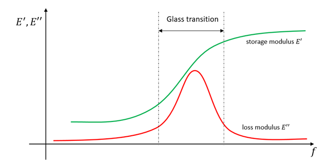
Figure 9: Typical behavior of a viscoelastic material with the frequency.

The loss modulus $E^”$ represents the damping properties of the material: the damping is very efficient in the so called ‘glass transition region’: the rubber must be chosen such that the frequencies to be damped will fall in the above region.  For this case, FEM analysis has shown that the first eigenfrequency of the system will be at around 700 Hz, therefore the rubber has been chosen taking this into account. Although the properties of a viscoelastic material are not defined for $f=0$, it is important here to estimate what will be the stiffness of the flexure assembly with quasi static loads (like thermal expansions for instance). From the data sheet of the material, the lowest frequency measured is 1,5 Hz. At this frequency the Young’s modulus is:

$E_r=8.08 MPa$

(4)

The shear modulus can be obtained by considering that for rubber the Poisson ratio is normally$v$≌0.5 :

$G_r=\frac{E_r}{2(1+\nu)}\approx \frac{E_r}{3}=2.7 MPa$

(5)

Equation (3) gives the stiffness of a single rubber sheet is, given the contact area  $S=697mm^2$ and thickness $h=2mm$.

$kr_x=9.4\:10^5 N/m$

(6)

The stiffness of the flexure assembly in $y$ is then:

$k_x=hf_x+2kr_x=5.67\:10^6 N/m$

(7)

As for the stiffness in the vertical direction $z$, the stiffness of the rubber is much higher than the one lateral direction, given by Equation (6). In fact, in this case the rubber works in compression, and given the ratio area/thickness the lateral contractions due to the compression must be considered contributing to the static stiffness: this increases stiffness of the rubber sheet remarkably. For a linear elastic material, the relation between stress and strain is defined by the equations of Navier:

$\epsilon_x=\frac{1}{E} \left(\sigma_x-\nu(\sigma_y+\sigma_z) \right) $      $\epsilon_y=\frac{1}{E} \left(\sigma_y-\nu(\sigma_x+\sigma_z) \right) $                 $\epsilon_z=\frac{1}{E} \left(\sigma_z-\nu(\sigma_x+\sigma_y) \right) $

(8)

Having the lateral contractions constrained it means that  $\epsilon_x = \epsilon_y =0$. Imposing this condition to the above system allows to express the relation between $\sigma_z$  and $\epsilon_z$:

   

$\frac{\sigma_z}{\epsilon_z}=E \frac{1-\nu}{2\nu^2+\nu-1}$

(9)

This equation allows to determine the vertical stiffness of the rubber sheet. Given that the Poisson ratio $\nu$ is not known exactly, a conservative value of $\nu=0.45$ will be chosen for this evaluation:

$\frac{\sigma_z}{\epsilon_z}=E \frac{1-\nu}{2\nu^2+\nu-1}$

(10)

As for the flexure contribution in $z$, the model of Figure 8 is still applicable:

$kf_z=2\frac{12EI_x}{L^3}=8.78 \:10^6 N/m$

(11)

The resulting stiffness is therefore:

$k_z=2kr_z+kf_z=4.2 \:10^7 N/m$

(12)

To recap, the flexure assembly is expected to have the following stiffness at very low frequency:

$k_x=5.67\:10^6N/m$	(13)
$k_y=2.1\:10^8N/m$	(14)
$k_z=6.3\:10^7N/m$	(15)

These values satisfy the requirements for the static stiffness.

Dynamic analysis: damping.

The positioning stage is a mechatronic system: in order to deliver high performance, low tracking and positioning error in combination with large accelerations or disturbances, the control system must have a minimum bandwidth of around 200 Hz. Initial simulations have shown that the first resonance is at a frequency of 700Hz, which is too low, limiting the bandwidth. The mode shape at 700 Hz shows a “decoupling” of the carrier and the chuck, so they move with respect to each other, generating significant deformation in $y$-direction. The structural stiffness could be increased a bit, and the mass lowered a bit by optimization, however this would not result in enough natural frequency increase to increase the control bandwidth to 200Hz. However, introducing enough damping will lower the peak of the bandwidth limiting resonance frequency, mitigating the instability at 200 Hz.

An initial calculation for the damper is setup, assuming deformations only in $y$, which will simplify the calculations, and provide an extra damping margin. Further optimization can be done in a later stage studying the actual mode shape (which will be influenced by the presence of damping) with FEM.

The analysis of the system transfer functions brings to set a requirement for the flexure assembly of a minimum damping such that the flexure assembly quality factor is $Q=13$ .  This corresponds to a relative damping of about 3%, at the frequency $f=700Hz$, in the direction $y$ was specified. From the definition of the Quality factor for structural damping, the loss factor of the system is:

$\eta=\frac{1}{\sqrt{Q^2-1}}=0.063$

(16)

As previously seen, the rubber pad and the flexure are working in parallel. Defining $k_r$ and $h_r$ the stiffness and the structural damping coefficient of the rubber pads, the flexure assembly can be modeled as shown in the below Figure 10:

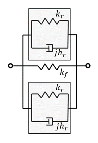
Figure 10: schematization of flexure assembly.

The loss factor (16) is not material property, but a property of the system. From the definition of structural damping:

   

$\eta=\frac{2h_r}{k_f+2k_r}$

(17)

The structural damping coefficient $h_r$ is a property of the rubber pad, and given that it works in shear it can be easily connected to the material property:

$\frac{h_r}{k_r}=\eta_r=\frac{E”}{E’}$

(18)

Expressing $h_r$ as a function of the material loss factor and replacing in (17):

$\eta=\frac{2k_r}{k_f+2k_r}\eta_r$

(19)

In order to meet the dynamic requirement, the following equation must be verified:

$\frac{2k_r}{k_f+2k_r}\eta_r \geq \frac{1}{\sqrt{Q^2-1}}=0.077$

(20)

For the chosen rubber, at the frequency of $700 Hz$ it is $\eta_r=1.371$ . Note that the stiffness of the rubber $k_r$  in the above equation (20) is not the same value used for the static analysis: at the frequency of $700 Hz$he rubber storage modulus is $E’= 47 \:MPa$ (about 6 times higher than the static value!), which brings the stiffness of the rubber at

$k_r=5.46\:10^6N/m$

(21)

Evaluating the first member of equation (20):

$\frac{2k_r}{k_f+2k_r}\eta_r =0.079 \geq 0.077$

(22)

Therefore the selected material in combination with the geometry satisfies the requirements.

Developed by

Hans van de Rijdt, Van de Rijdt Innovatie.

Francesco Patti, VDL ETG.

Reference:

–