4.2 Lumped capacitance modeling
In this chapter the Lumped capacity model is explained, including calculation steps.
In a lumped capacitance model, a thermal system is divided into:
- Heat Capacitances
- Thermal Couplings
The heat capacities are individual parts of the system which can be considered to be at uniform temperature, while under influence of the thermal couplings. In other words, the heat capacities are parts of the system which have low Biot numbers. Some parts parts which have high Biot numbers may be split into smaller pieces, connected to each other by a thermal coupling, such that the Biot number of individual pieces is sufficiently low (Bi << 1). The thermal couplings would be determined by the internal (Fourier) heat conduction in the part.
Thermal couplings connect the heat capacities. They can be conduction, radiation, convective or contact couplings. A thermal coupling may consist of a physical part of the system, especially if its Biot number is high ( Bi >> 1), and its heat capacity is low compared other parts of the system.
The result is a network of nodes (heat capacities) interconnected by thermal couplings. The thermal couplings allow the nodes to exchange heat between each other. The rate of heat exchange between 2 individual nodes is a simple matter of Q = TC*ΔT. The network of nodes and thermal couplings results in a system of these equations, which can be solved using linear algebra. Here, we’ll use a ready-made Mathcad template for the calculations, but the set-up of the problem (which is as important as the calculation itself) is the same, regardless of the calculation tool that is used.
Setting up the model
Step 1: Define the heat capacities
First, the heat capacities (nodes of the thermal network) need to be determined. Individual heat capacities can be:
- Large parts (high heat capacities, large time constants)
- Thermally conductive parts (Parts with Biot<<1)
- Group of parts with good thermal conduction between them
- Sections of parts (if internal conduction low (Biot>1) split it up in smaller parts)
- Parts with “important” temperatures
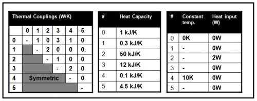
Next, number individual heat capacities (or “nodes”), starting from 0. Then calculate the total heat capacity (J/K) for each node and enter the results into a table. Below is an example table for a system with 6 nodes.
| Node # | Heat capacity |
| 0 | 1000 J/K |
| 1 | 300 J/K |
| 2 | 50000 J/K |
| 3 | 12000 J/K |
| 4 | 100 J/K |
| 5 | 4500 J/K |
Step 2: Define the thermal couplings
Identify thermal couplings between nodes in the system. A single thermal coupling always acts between 2 nodes. Thermal couplings are typically:
- Small Connecting parts (Low heat capacities, small time constants)
- Poorly conducting parts (Parts with Biot>>1)
- Heat Conduction within a split part
- Radation couplings between large surface areas
- Thermal contact conductances
- Convective heat transfer between two parts
Next, calculate the total thermal coupling between each pair of nodes. In case there is more than one coupling between 2 nodes, calculate the total as follows:
Two or more couplings in a parallel configuration:
- TCtotal=TC1+TC2 + …
Two couplings in a series configuration:
- 1/ TCtotal =1/TC1+1/TC2 + …
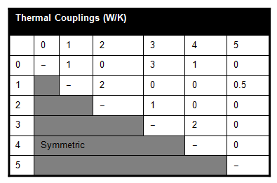
Finally, enter the results into a square matrix, of which each row and each column corresponds to a node. So, row 2, column 3 of the matrix contains the total thermal coupling between nodes 2 and 3. Of course, this matrix is symmetric. An example matrix is shown below. It shows that the thermal coupling between nodes 2 and 3 is 1 W/K.
Step 3: Define boundary conditions
Boundary conditions are the heat inputs and outputs of the system. These are:
- Nodes with a constant (known) temperature
- Heat sources within nodes
Enter the boundary conditions into a table. Below is an example:
| Node # | Constant Temperature (K) | Heat input (W) |
| 0 | 0 K | 0 W |
| 1 | – | 0 W |
| 2 | – | 2 W |
| 3 | – | 0 W |
| 4 | 10 K | 0 W |
| 5 | – | 0 W |
Step 4: Enter the input in the template
The information collected in the tables can be entered in a template (eg Calculator: Lumped mass – steady state.) The actual calculation of the lumped capacitance model is the solution of a system of equations.
There are two basic equations:
- Q=TC* ΔT heat flow through a coupling
- T/dt = ΣQ/C Total heating rate of a node
So, for each node there is an equation:
- dT/dt=Σ(TC* ΔT ) /C
These equations (one for each node), make up a system of (differential) equations, with boundary conditions as given. The steady-state solution gives the temperatures of the nodes and heat flow rates through the couplings after the system has reached equilibrium (that is, when dT/dt = 0 in the equation above). The time-dependent solution shows how the thermal system evolves (toward its equilibrium) in time. The Calculator Lumped mass – Transient calculates each of these solutions.
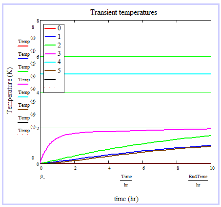
Example results
The template returns steady-state results, and transient (time-varying) results in graphical form. If the heat capacities are not entered, only the steady-state result is returned (this result is independent of heat capacities). The results for the examples used above are shown here.